ELCOME dear friends of electrical engineering. In our new, exciting technical article, A. Eberle GmbH & Co. KG explains the control options for electric coils. Have fun reading, we're handing over!
E-coil control - Resonance & Location Curve Procedure
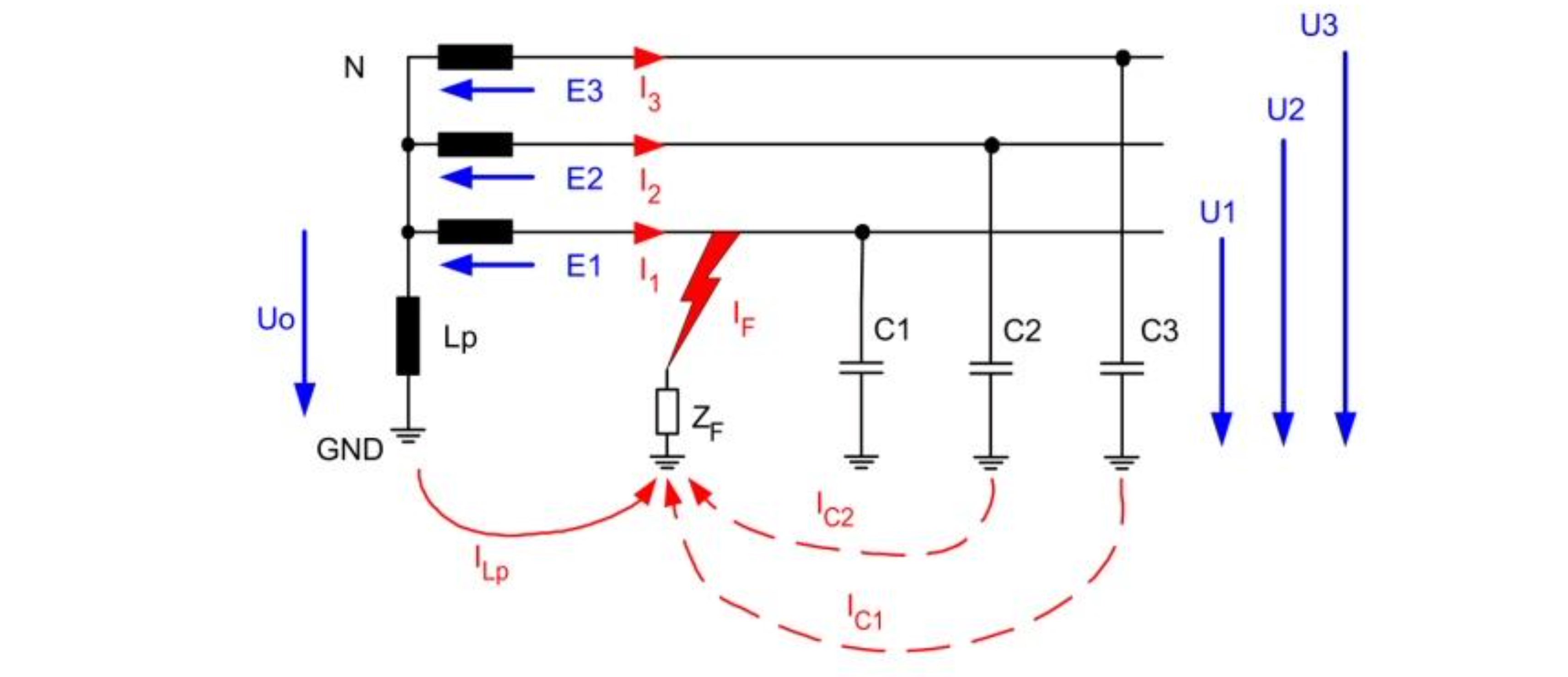
In "compensated networks" the current through the point of failure is minimized with the help of an earth fault compensation coil (e-coil). For this purpose, the e-coil is already in operation in a healthy network, i.e. set without an earth fault so that in the event of an earth fault, the capacitive component of the current is compensated by an inductive current through the fault location. The following figure, Figure 1, shows the network in the case of a single-pole earth fault in Phase L1.

The objective of the e-coil control is now to set the e-coil in the healthy network operation to the desired value already. Several methods are available for the control, wherein the equivalent circuit for the resonance procedure and the location curve procedure can be derived without the use of symmetrical components.
Simplified equivalent circuit
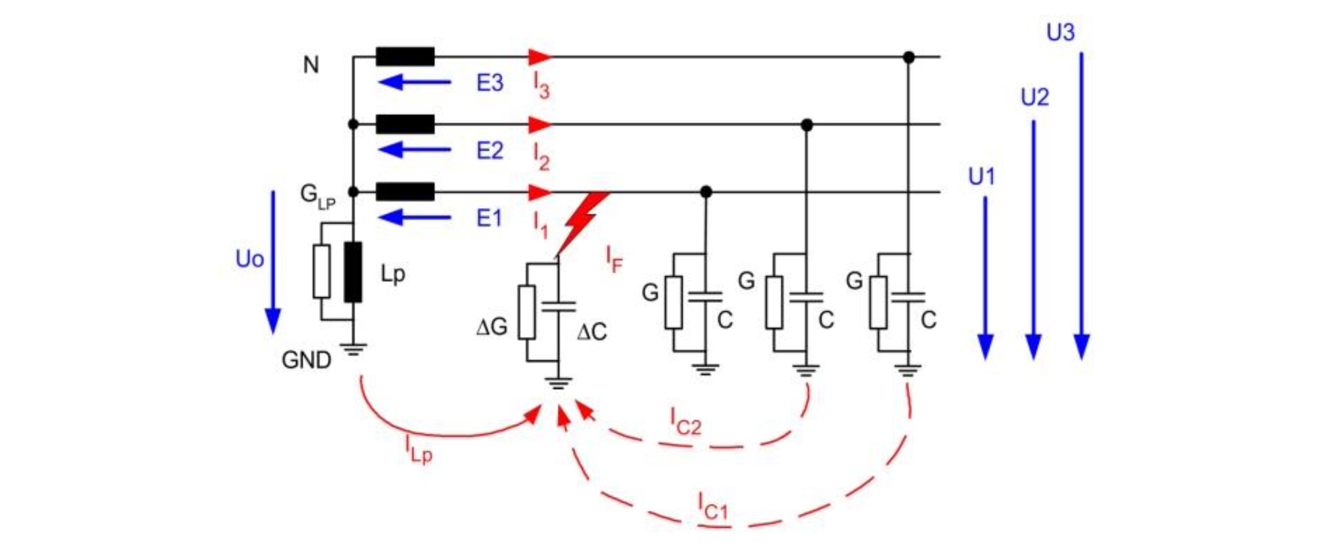
The simplified equivalent circuit diagram should describe the network in the range from the operating state "healthy network" to the operating state "saturated earth fault". First, for a simpler notation, the capacitances of the network and the inductance of the e-coil are replaced by their complex conductances (admittances). It is assumed that the resistive or capacitive asymmetry in the case of an saturated earth fault is present in only one phase:
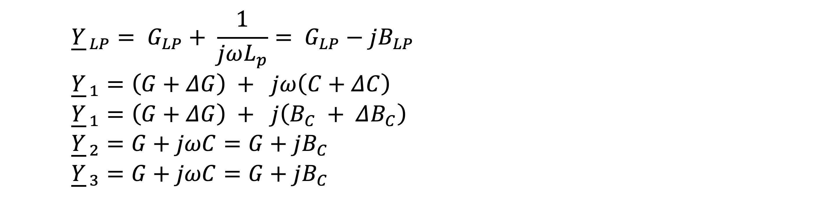
For the neutral point N of the transformer, the following nodal equations can be specified:

If the currents from the following mash equations
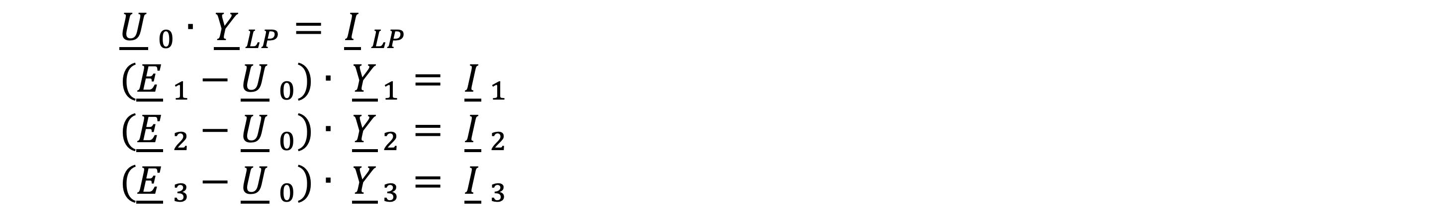
are used in the nodal equation for ILP, this yields the following equation:

It is assumed that a symmetrical three-phase network is present, then the phase voltages E2 and E3 are construed as the phase voltages E1 rotated by 120 degrees. This rotation by 120 degrees can be described by the complex operator a:

The voltages E2 and E3 are thus:

Furthermore, the sum of the three voltages is zero:

Since E1 corresponds to the phase voltage and is no equal to 0, the following also applies:

If the voltages E2 and E3 are replaced in the above equation Uo · YLP =... and the coefficients combined, we get the following equation:

or, after conversion, the voltage divider equation

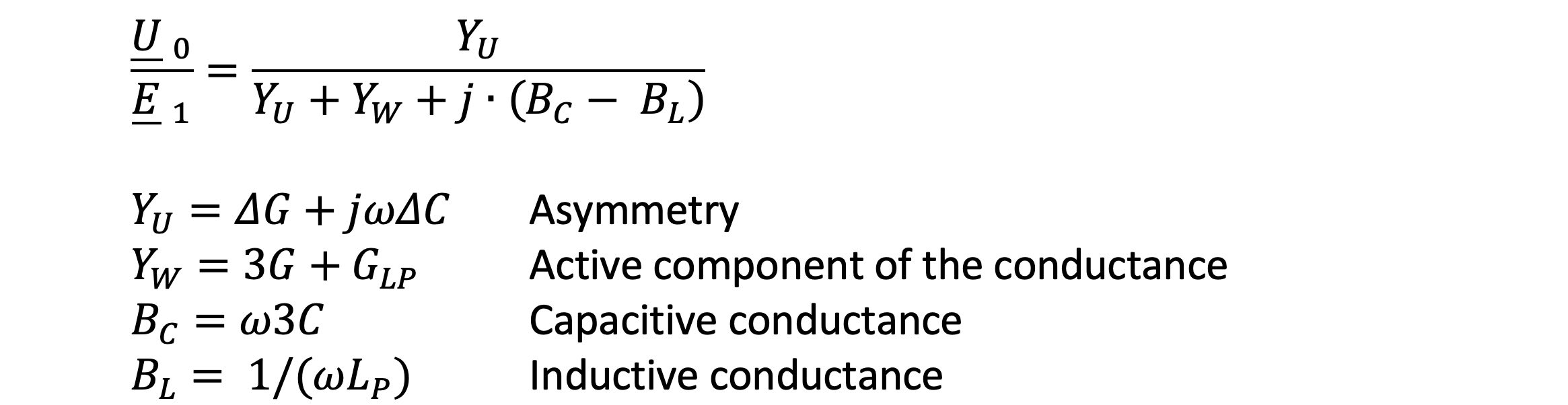
If parts of the equation are again considered in their full expression, the result is the following equations:
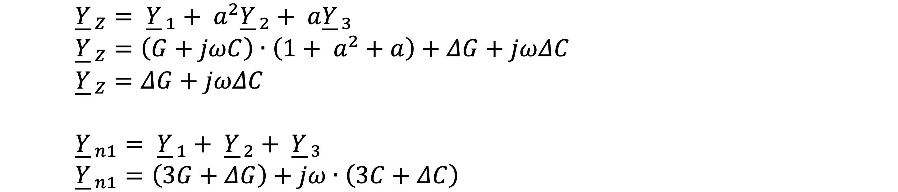
If these admittances (admittances) and YLP are again inserted into the voltage divider equation and the coefficients summarized, we obtain the following expression:
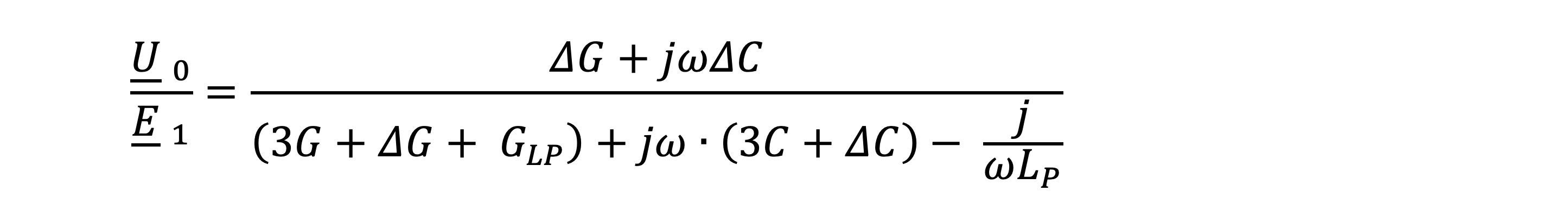
The coefficient compared to the voltage divider equation
Thus, the following simple equivalent circuit can be drawn.
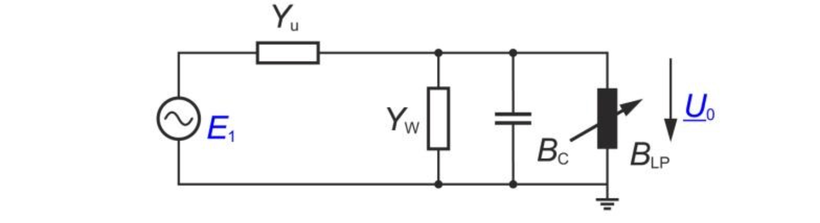
This equivalent circuit describes the earth fault compensation in both "healthy operation" and in the case of an "earth fault". In a healthy network, the complex conductance of the asymmetry Vu is very small, i.e. the asymmetry is considered to be a very high resistance impedance. In the earth fault on the other hand, G is very large so that ωC can be ignored. This corresponds to a low-resistance earth fault.
If we start with the equation with a constant network status
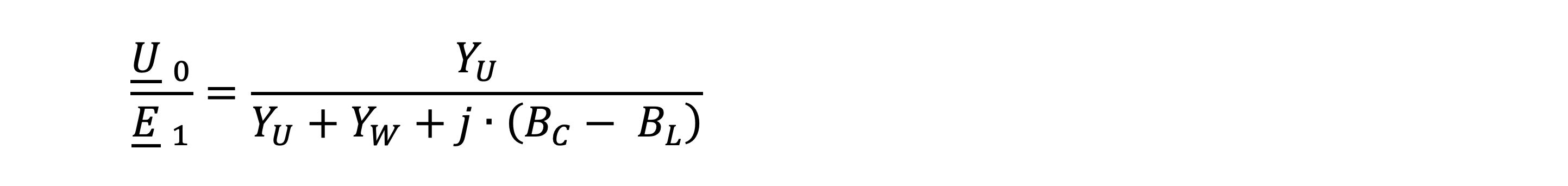
the setting of the e-coil and thus of the susceptance BL changes, then the voltage dividing ratio is changed based on the phase voltage E1. If the value of the zero sequence voltage applied to the coil position is plotted, the result is the "resonance curve".
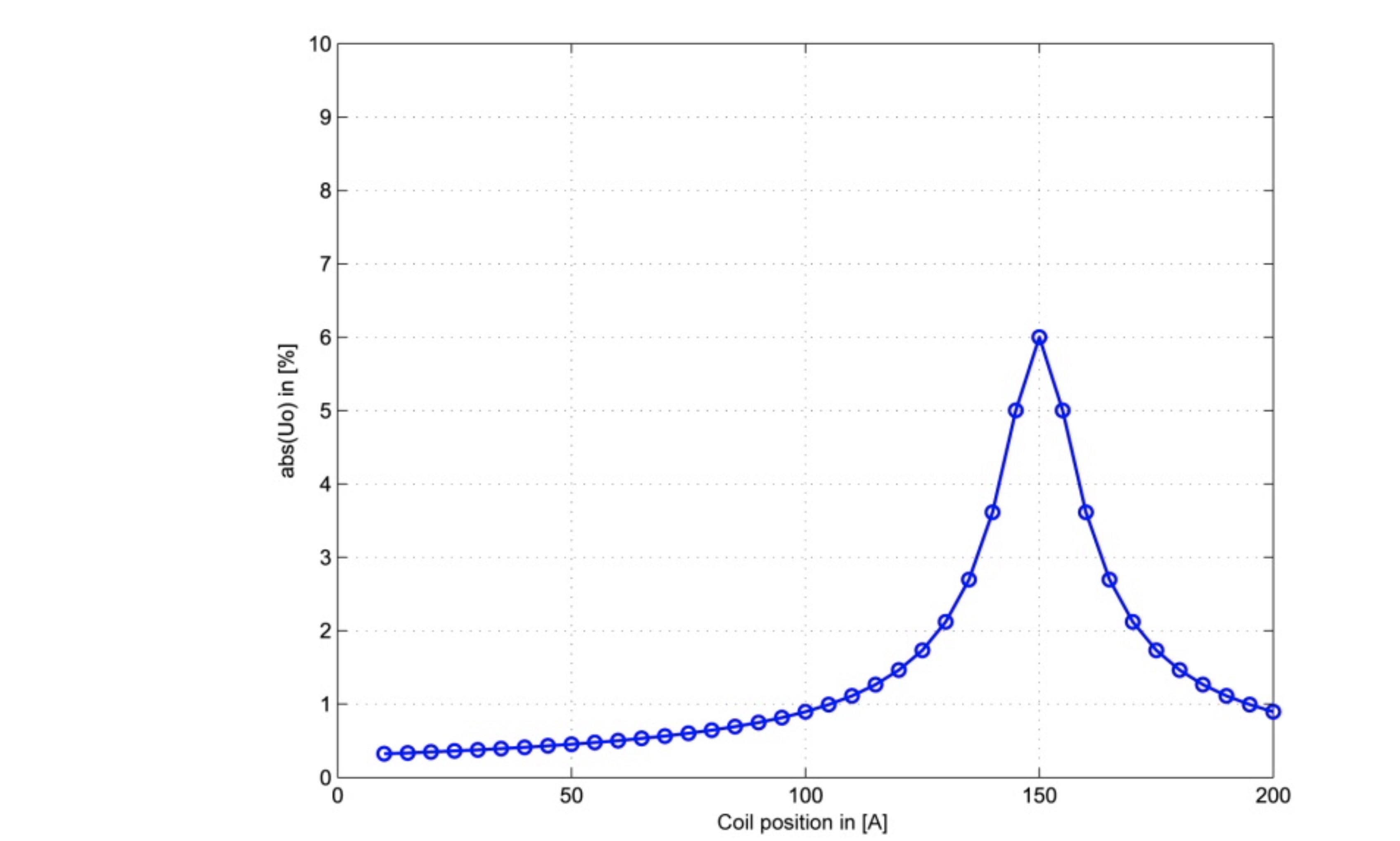
The zero sequence voltage is greatest when the susceptances cancel the denominator. In this case, the system is tuned. In other cases, either a capacitive or inductive component is added, so that the zero sequence voltage becomes smaller.
In practice, the zero sequence voltage Uo is usually plotted logarithmically to detect even small values of Uo and its changes.
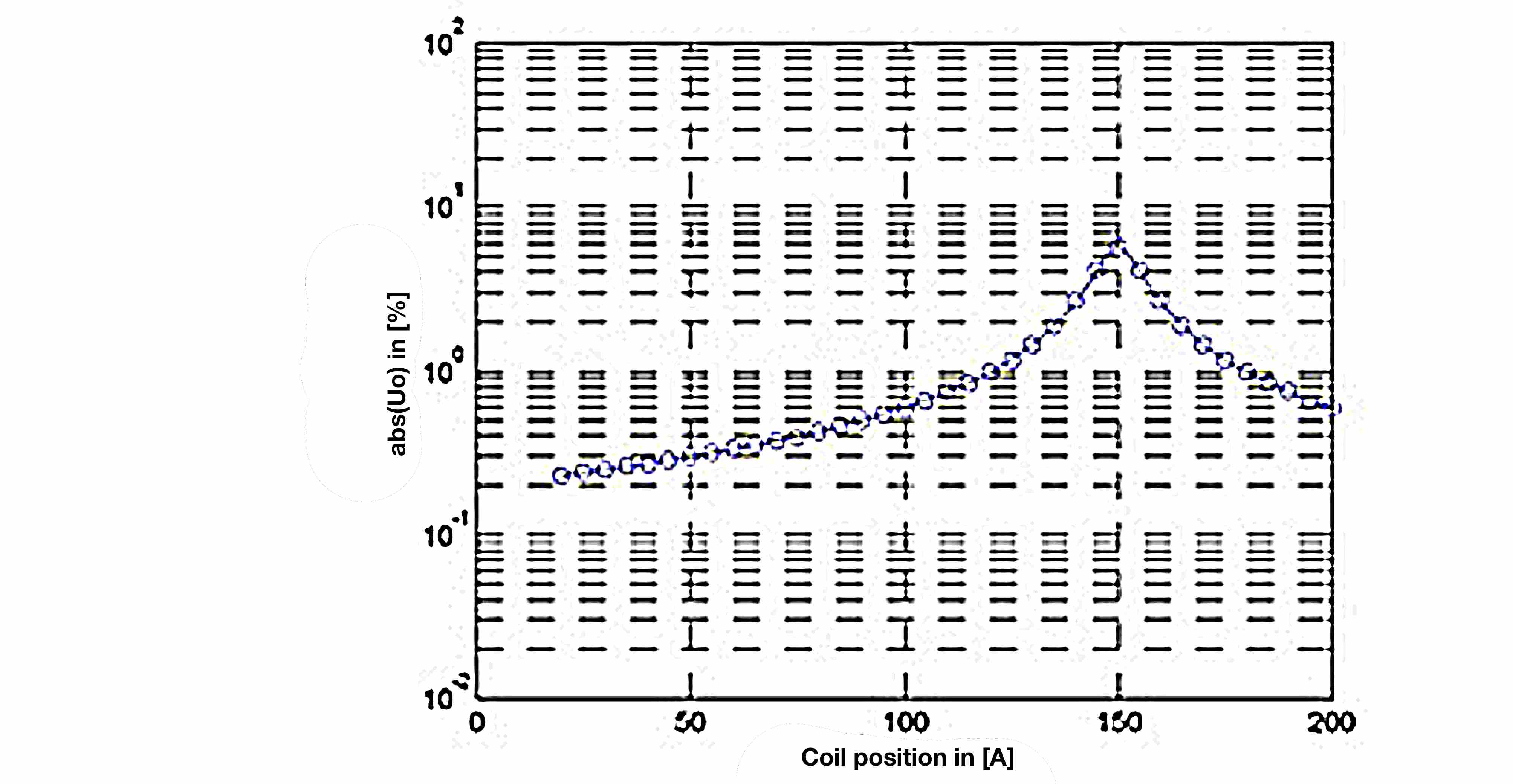
The inductance of the e-coil is usually specified only indirectly, namely in [A]. In practice, the inductance is not interesting, but what compensation current in the case of a saturated earth fault is made available through the e- coil. For this reason, the display of e-coil position is calibrated in [A].
The actual current flowing through the e-coil in the event of an earth fault depends on the fault resistance and in case of a high-resistance earth fault is substantially smaller.
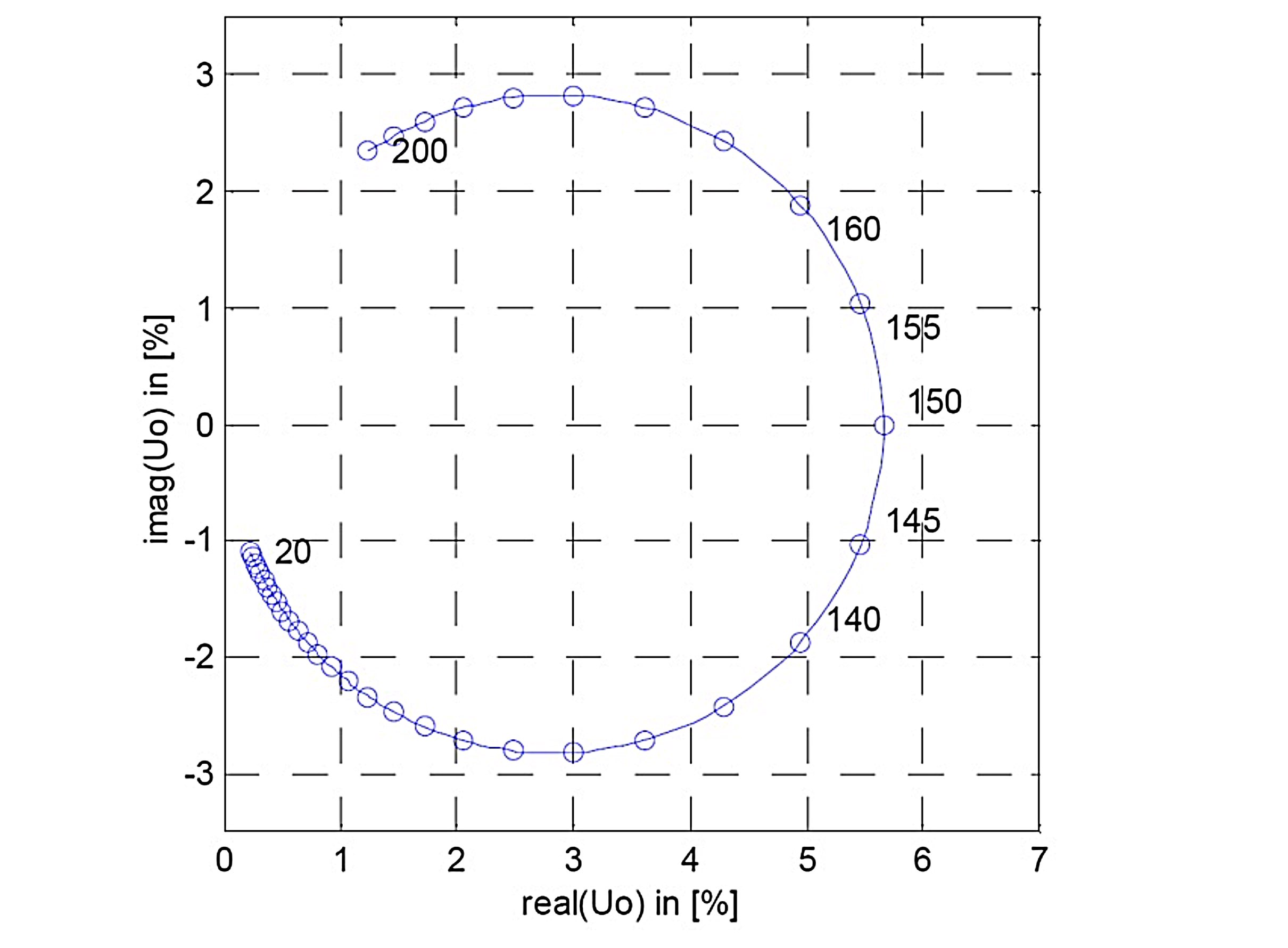
Another representation of the resonance curve is obtained when the residual voltage Uo is plotted on a linear scale according to the value and angle. In this case we obtain the location curve of Uo. The angle of Uo refers to the phase voltage E1, which corresponds to the single-phase voltage, in which the asymmetry is assumed.
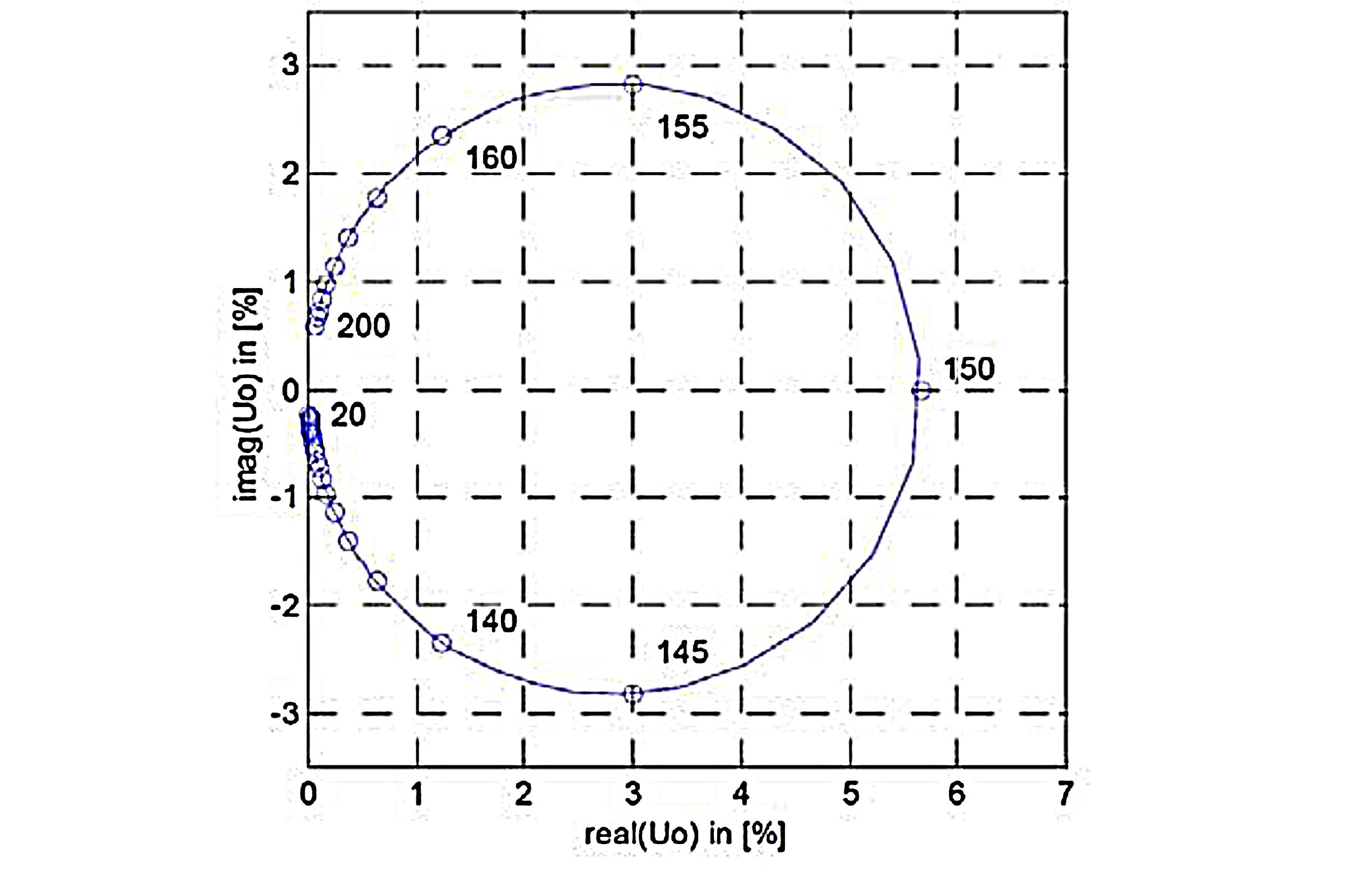
In the location curve representation the coil position itself is not directly visible. The coil position is only available as a parameter for individual points. In the above representation, the associated spool position has been added at some points.
The resonance curve or location curve can be clearly described, among other things, by the following parameters:
Ures - Maximum zero sequence voltage Uo at the resonance point
Ires - Coil setting at which the maximum resonance Ures of the zero sequence voltage Uo occurs.
d - Damping of the resonant circuit
The attenuation of an oscillating circuit is defined by the following equation:
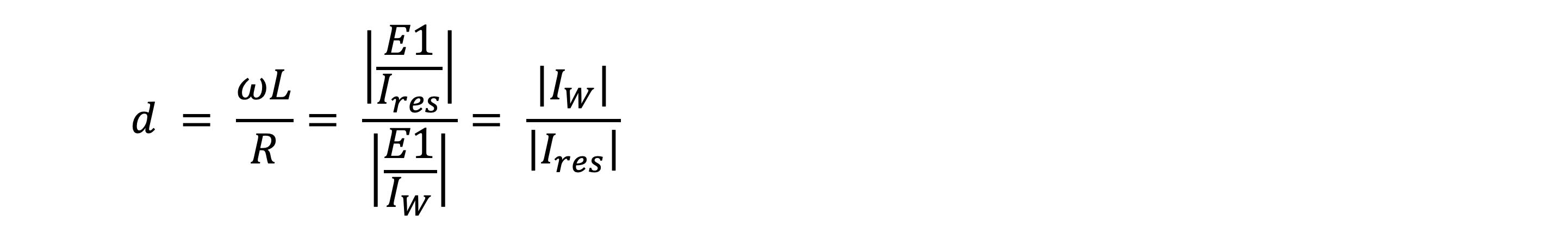
The value of the loss or the expected active current in the event of a saturated earth fault can be determined directly from the resonance curve. This requires that each spool position Id is searched for wherein the ratio of the value of the zero sequence voltage is due to

Justification:
In general, for Uo:
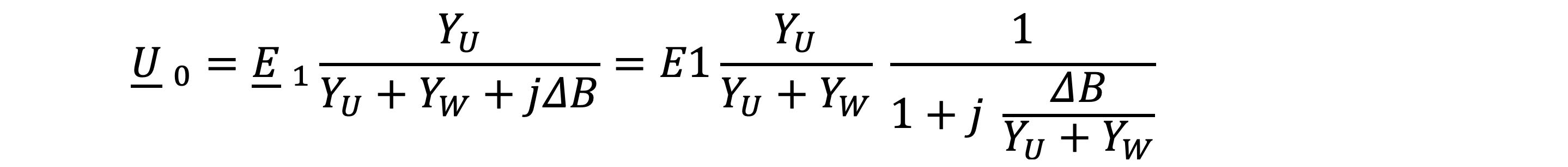
With ideal tuning ∆B = 0, so that for Ures at the resonance point, the following equation applies:

Used in the above equation this gives:
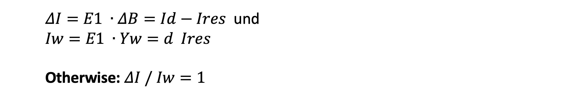
It follows from this that at this point the value of the fault tuning of the susceptances ∆B is equal to the value of the active component (Yw+Yu) is. At the point considered is Yu << Yw, so Yu can be ignored. If the conductance is calculated from the currents with the help of the phase voltage E1 flows, this gives
After division of the equations and multiplying by d on both sides, this gives:
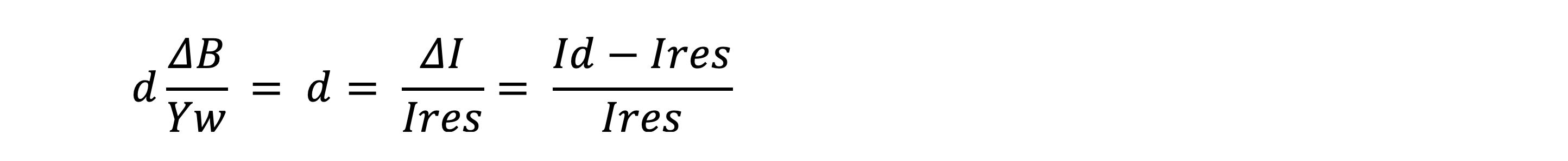
The damping thus describes whether the response curve is flat or steep and on the other hand gives the minimum current through the point of failure in the case of a saturated earth fault. A flat response curve therefore indicates a large attenuation and a large active current through the point of failure. Conversely, a steep response curve indicates a small attenuation and a small active current through the point of failure.
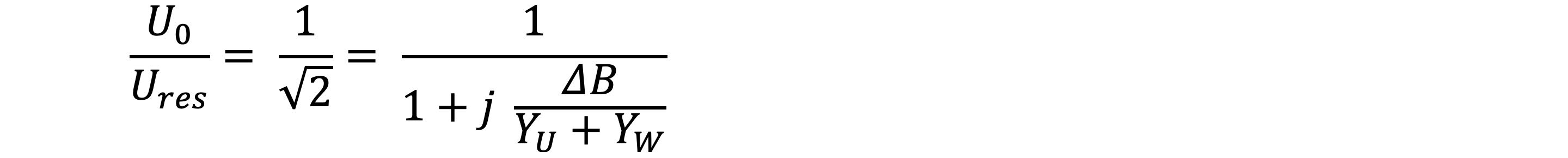
In the location curve representation, the associated current values can found at an angle of ±45°. On these points, the value of Uo is only 1/√2 related to Ures.
The following figures show the same network with a stronger damping and the same resonance point (Ures, Ires) as before:
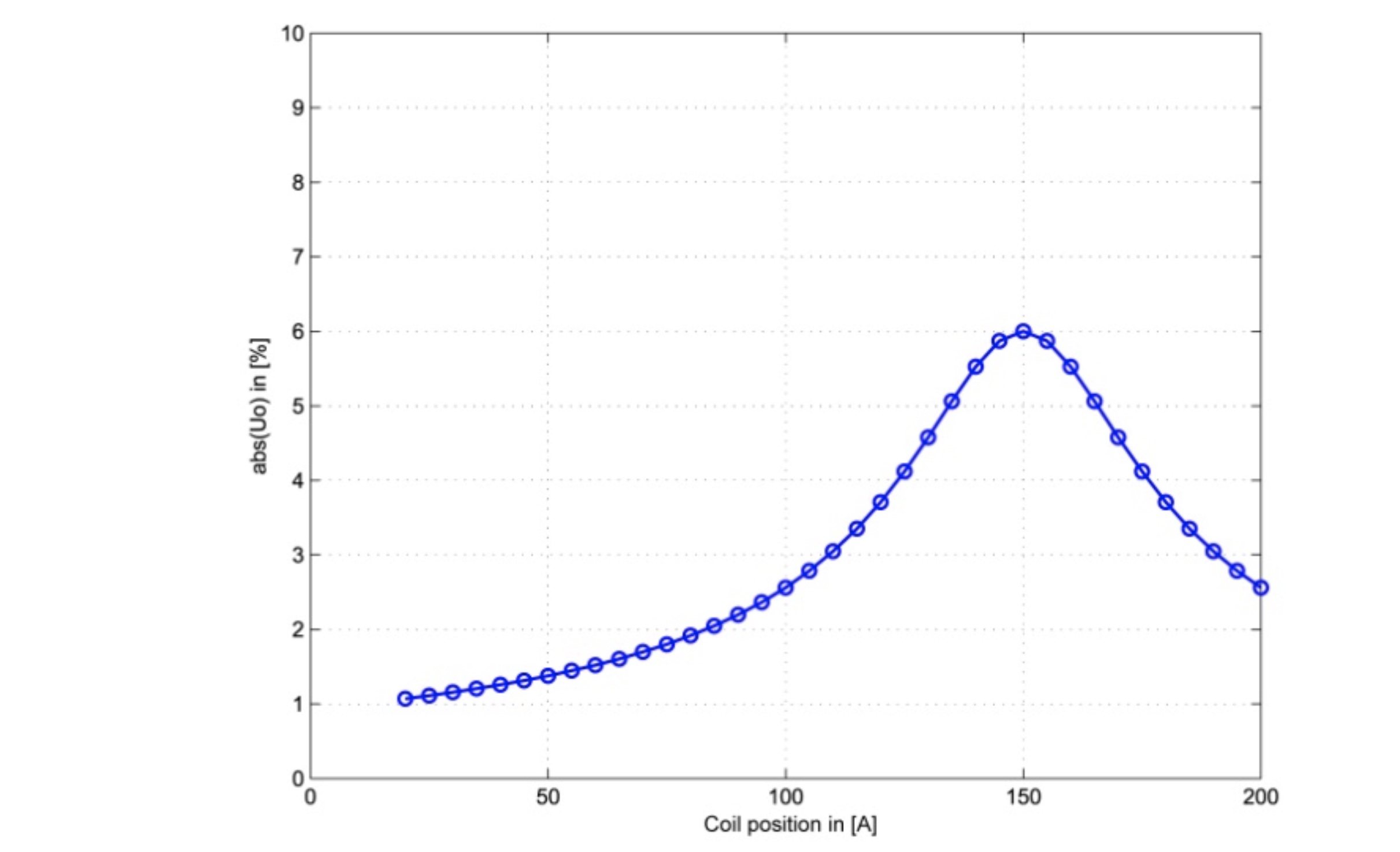
It can be seen that the resonance curve is substantially flatter. The damping d = 25 A is directly readable at a zero sequence voltage of 4%.
In the location curve representation it can be seen that the change in angle between the individual coil positions is substantially less.
Pros and Cons:
The realization of the measurement of the value of a voltage, as used in the resonance curve procedure, is relatively non-critical and can be performed up to the range of a few mV with sufficient accuracy. Since the control of the earth fault compensation performs a tuning at 50 Hz, for the measurement of Uo a 50 Hz filter is connect upstream.
In the determination of the location curve, a much higher cost in the measurement is necessary because, in addition, the angle of Uo can also be determined for very small voltages. This requirement is especially true for points that are not in the vicinity of the resonance point. Additionally a misalignment of the upstream 50 Hz filter has a much greater effect.
Author: Dr. Gernot Druml
Kind regards
your EEA-Team